| This text was taken from
P.A.Wozniak, Economics of learning, Doctoral
Dissertation, University of Economics, Wroclaw, 1995
and adapted for publishing as an independent article on the Web. (P.A.Wozniak, Aug 21,
1998) For a similar study on the relationship between the IQ and the learning process see: Investigating the correlation between the intelligence and the performance in repetitive learning tasks |
Working together with Dr. Gorzelañczyk from Medical Academy of Poznañ, I have subjected a number of high school students to a long-term learning process with the use of a uniform database, uniform working conditions, equal learning process duration and Algorithm SM-6 for spaced repetition based on approximating forgetting curves and making use of the concept of the forgetting index. The experiment is now in its third year [this text was written in 1994, the experiment continues in 1998], and data from over 30 students have been collected providing a unique opportunity to compare all learning parameters taken from students’ computer record files.
Similar, though much less uniform experiment, and on a smaller scale, has been conducted four years ago with the use of Algorithm SM-5 based on the direct modification of optimal factor matrices (Wozniak et al. 1994). The cumulative data from this earlier experiment has been used to determine the initial values of the entries in the optimal factor matrix used in Algorithm SM-6.
Subjects. The subjects were 32 volunteers, high school students, aged 18-20.
Material. 2500-item list of questions and answers related to biology material required at entrance examinations for Medical Academy in Poland (in Polish). For example:
- Question: Which blood group makes up a universal donor?
- Answer: 0
Procedure. All subjects used Algorithm SM-6 for spacing repetitions and implemented in SuperMemo for Windows. The working time was 2-3 times a week from 20 to 50 minutes in a single session. The entire list of questions and answers was memorized within 2-3 months in a self-paced manner. Later, repetitions of the memorized knowledge continued for 6-7 months. All parameters of the learning process, including the parameters of the algorithmic procedure have been collected in computer files. Statistical analysis tools have been used to interpret the data as specified in each particular presented case.
Remarks. Not all subjects fully complied with requirements set before the experiments in reference to: (1) number of memorized items, (2) regularity of learning sessions, and (3) length of the post-memorization period. Consequently, only 20 data records have been selected for final analysis.
Before I step toward the statistical comparison of subjects’ learning process, I would like to present some interesting observations that have been made in reference to the possible causes of the differences between particular students. As Dr. Gorzelañczyk was personally involved in supervision of the learning process as well as in tutoring of the subjects on relevant topics, I asked him to grade each of the subjects with respect to general intelligence and attitude towards learning. Naturally, such grading is always greatly biased by subjective judgment of the supervisor; nevertheless, I considered it an important source of possible conclusions. The grading of intelligence did not show significant correlation with any of the parameters of the learning process measured in the experiment [see: Correlation between the intelligence and the retention in learning based on repetition spacing (Gorzelanczyk et al., 1998)]. However, I was able to use the results of entrance examinations of all the subjects as a general bench mark of the overall performance (all the subjects were candidates for students at Medical Academy of Poznañ). A very interesting and surprising conclusions could be drawn from the correlation analysis on the learning-performance platform.
It is a common sense reasoning that good students learn faster than bad students; the fact that should be reflected by the parameters of the learning process. A natural intuition is that good students should exhibit low forgetting index, quick response time, high grades, etc.
My observation is, however, that in learning based on self-assessment, the opposite correlation appears to be true. Successful students apparently learned slower and appeared to forget items much more frequently than the unsuccessful students!
The interpretation of this paradoxical finding is that good students are by far more critical in the judgment of their own progress. It has been for long postulated in my earlier publications that there is very little difference between individuals as far as the mechanisms of memory are concerned. It is the way humans process information that sets them apart from each other. Consequently, little difference could be observed among the students in the ability to remember. However, those who appeared to be self-indulgent and lenient in self-assessment, usually showed much lower levels of knowledge retention in absolute terms (i.e. as judged by the supervisor).
The following general parameters of the learning process have been collected from the subjects in the course of the experiment (cf. Table 1 Comparison of learning parameters in a group of 20 subjects):
- Day - the number of the day of the learning process on which repetitions stopped (from 178 to 266 days)
- Total - total number of items in the database (this number may differ because of two reasons: (1) subjects were allowed to delete items, (2) the list of questions increased in size in the second year of the experiment by about 400 items
- Memorized - total number of memorized items in the database
- Intact - number of items that have not been memorized
- Outstand - number of items that have been outstanding for repetition on the day the measurements were taken (large number of outstanding items comes from the fact that the most recent data logging took place as late as 17 months after ceasing repetitions)
- Burden - average number of items scheduled for repetition per day at the moment of ceasing repetitions, computed as the sum of interval reciprocals (from 9 items/day to 102 items/day!)
- Time - average repetition time in seconds (notably, the differences between subjects in the time in which they provide the response are as 1:16; from 0.52 sec/item to 8.73 sec/item)
- Workload - total daily repetition time in minutes (from 0.09 min/day to 5.9 min/day; here the difference is like 1:65!)
- Interval - average inter-repetition interval in the database at the moment of taking the measurement (in days; from 115 days to 351 days)
- Factor - average E-factor in the database (from 2.464 to 2.706) [The concept of E-factor in Algorithm SM-6 corresponds roughly to A-factors in Algorithm SM-11]
- Rep - average number of repetitions that have been made per item (from 2.29 to 3.36)
- Day/Rep - average inter-repetition interval in the database until the moment of taking the measurement (in days; from 58 to 90 days; same as Entry 1 divided by Entry 11 in the table)
- Number of times an average item has been forgotten (from 0.01 to 0.65)
- FI req - requested value of the forgetting index
- FI det - detected value of the forgetting index in the database, which, in the ideal case, should equal the requested value listed in Entry 14 (from 0.3% to 19.4%)
- FI cas - repetition cases used to compute the value FI det (Entry 15), i.e. the total number of repetitions made by a given subject (from 2906 to 8209)
- Grade - trailing average of grades provided during recent repetition sessions on the grade point scale from 0 to 5, where 5 is best (from 4.12 to 4.999)
- Last - the month and year of the latest repetition in the schedule (from May 1994 till April 1996)
- 1.3s - number of items with E-factor equal to 1.3 (from 0 to 19)
- Dif 1, Dif 2 and Dif 3 - weighted average of differences between neighboring entries in the matrix of optimal factors for repetitions numbered one, two and three respectively (the difference between neighboring entries is OF[EF,R]-OF[EF-0.1,R] where EF is E-factor and R is repetition number)
- OF x y - selected entries of the matrix of optimal factors (e.g. OF 1.3 1 indicates the entry corresponding to E-factor equal to 1.3 and the repetition number equal to one)
| File | AGNIE | ANI | EWA | IZA | KARF | MARCI | MARYS | OLA2 | OLA1 | AGA |
| Day | 232 | 178 | 186 | 198 | 244 | 241 | 242 | 192 | 256 | 240 |
| Total | 2449 | 2449 | 2449 | 2449 | 2449 | 2449 | 2449 | 2449 | 2449 | 2859 |
| Memoriz | 2449 | 1743 | 1954 | 1954 | 1104 | 2449 | 2449 | 1996 | 2449 | 2859 |
| Intact | - | 706 | 495 | 495 | 1345 | - | - | 453 | - | - |
| Outstand | 2449 | 1743 | 1954 | 1954 | 1104 | 2449 | 2449 | 1996 | 2449 | 588 |
| Burden | 36.09 | 40.33 | 20.01 | 30.58 | 10.64 | 45.91 | 102.43 | 30.49 | 60.81 | 9.04 |
| Time | 3.58 | 6.71 | 4.16 | 4.20 | 4.65 | 5.74 | 3.22 | 8.73 | 5.86 | 3.84 |
| Workld | 2.15 | 4.51 | 1.39 | 2.14 | 0.82 | 4.39 | 5.49 | 4.44 | 5.94 | 0.58 |
| Interval | 196 | 119 | 125 | 123 | 139 | 175 | 116 | 115 | 156 | 351 |
| Factor | 2.618 | 2.509 | 2.574 | 2.558 | 2.556 | 2.606 | 2.517 | 2.604 | 2.627 | 2.689 |
| Rep | 2.58 | 2.46 | 2.29 | 2.87 | 3.29 | 2.74 | 3.30 | 2.97 | 3.10 | 3.11 |
| Day/Rep | 89.9 | 72.3 | 81.2 | 68.9 | 74.1 | 88.1 | 73.3 | 64.6 | 82.4 | 77.2 |
| Lapses | 0.08 | 0.35 | 0.14 | 0.32 | 0.42 | 0.12 | 0.65 | 0.26 | 0.24 | 0.01 |
| FI req | 10 | 10 | 10 | 10 | 10 | 10 | 10 | 10 | 10 | 10 |
| FI det | 5.03 | 18.28 | 9.67 | 13.85 | 14.61 | 6.26 | 19.44 | 10.89 | 9.62 | 0.31 |
| FI cas | 4231 | 3370 | 2906 | 4534 | 3169 | 4582 | 8209 | 4676 | 6061 | 5845 |
| Grade | 4.904 | 4.122 | 4.844 | 4.393 | 4.907 | 4.777 | 4.798 | 4.691 | 4.904 | 4.979 |
| Last | 11.94 | 05.94 | 06.94 | 07.94 | 08.94 | 09.94 | 08.94 | 06.94 | 10.94 | 03.96 |
| 1.3s | - | 4 | - | 10 | - | - | 17 | 4 | 1 | - |
| Dif 1 | 1.21 | 0.30 | 1.01 | 0.43 | 0.03 | 0.64 | 0.17 | 0.46 | 0.54 | 1.44 |
| Dif 2 | 0.25 | 0.04 | 0.21 | 0.28 | -0.01 | 0.24 | 0.12 | 0.15 | 0.18 | 0.31 |
| Dif 3 | 0.13 | 0.10 | 0.12 | 0.04 | 0.10 | 0.11 | -0.00 | 0.08 | 0.09 | 0.13 |
| OF 1.3 1 | 5.46 | 4.07 | 7.56 | 2.76 | 9.70 | 5.43 | 2.15 | 1.72 | 1.46 | 2.75 |
| OF 1.3 2 | 1.86 | 2.32 | 2.09 | 1.33 | 3.06 | 2.01 | 1.24 | 2.69 | 2.25 | 1.26 |
| OF 1.3 3 | 1.39 | 1.40 | 1.39 | 1.53 | 1.65 | 1.53 | 1.88 | 1.59 | 1.82 | 1.33 |
| OF 2.5 1 | 19.97 | 7.65 | 19.64 | 7.93 | 10.00 | 13.14 | 4.25 | 7.26 | 7.90 | 20.00 |
| OF 2.5 2 | 4.90 | 2.75 | 4.67 | 4.65 | 2.91 | 4.94 | 2.72 | 4.45 | 4.36 | 5.00 |
| OF 2.5 3 | 2.92 | 2.62 | 2.81 | 2.07 | 2.80 | 2.90 | 1.85 | 2.50 | 2.94 | 2.89 |
| File | KAR | KASI | KASK | MAG | MIKO | MONI | OLA3 | SEBA | TOMA | NATA | Aver | Total |
| Day | 184 | 246 | 235 | 237 | 245 | 248 | 232 | 264 | 250 | 266 | 232 | - |
| Total | 2866 | 2859 | 2859 | 2859 | 2859 | 2859 | 2859 | 2788 | 2859 | 2859 | 2687 | 53426 |
| Memor | 2866 | 2859 | 2859 | 2859 | 2859 | 2859 | 2859 | 2788 | 2859 | 2859 | 2526 | 49932 |
| Outst | 725 | 567 | 918 | 1154 | 1123 | 754 | 838 | 641 | 459 | 916 | 1314 | 27230 |
| Burden | 10.45 | 9.70 | 11.14 | 11.76 | 13.06 | 10.43 | 11.11 | 9.18 | 9.68 | 12.55 | 23.60 | 495.37 |
| Time | 0.52 | 4.33 | 5.01 | 3.45 | 2.04 | 2.19 | 5.02 | 1.14 | 4.70 | 3.38 | 4.05 | - |
| Workl | 0.09 | 0.70 | 0.93 | 0.68 | 0.44 | 0.38 | 0.93 | 0.17 | 0.76 | 0.71 | 1.77 | 37.63 |
| Intervl | 301 | 324 | 292 | 295 | 249 | 313 | 323 | 332 | 324 | 272 | 238 | - |
| Factor | 2.706 | 2.598 | 2.667 | 2.464 | 2.618 | 2.680 | 2.673 | 2.684 | 2.679 | 2.608 | 2.618 | - |
| Rep | 3.14 | 3.10 | 3.07 | 3.36 | 3.10 | 3.02 | 3.01 | 3.03 | 3.01 | 2.95 | 2.98 | - |
| Day/R | 58.5 | 79.4 | 76.5 | 70.6 | 78.9 | 82.1 | 77.1 | 87.2 | 83.1 | 90.3 | 77.8 | - |
| Lapses | 0.01 | 0.01 | 0.05 | 0.18 | 0.16 | 0.05 | 0.05 | 0.03 | 0.04 | 0.16 | 0.16 | - |
| FI req | 10 | 10 | 10 | 10 | 10 | 10 | 10 | 10 | 10 | 10 | 10 | - |
| FI det | 0.37 | 0.43 | 2.36 | 7.03 | 6.84 | 2.55 | 2.48 | 1.50 | 1.81 | 7.48 | 6.71 | - |
| FI cas | 6177 | 6029 | 6113 | 7458 | 6549 | 5992 | 5937 | 5745 | 5869 | 6081 | 5534 | 109 K |
| Grade | 4.991 | 4.746 | 4.977 | 4.953 | 4.999 | 4.908 | 4.623 | 4.998 | 4.998 | 4.910 | 4.829 | - |
| Last | 11.95 | 03.96 | 02.96 | 02.96 | 01.96 | 02.96 | 02.96 | 04.96 | 02.96 | 02.96 | - | - |
| 1.3s | - | - | - | 19 | - | - | - | - | - | - | 3 | 55 |
| Dif 1 | 1.42 | 1.43 | 1.18 | 1.18 | 0.47 | 1.29 | 1.44 | 1.11 | 1.32 | 0.95 | 0.93 | - |
| Dif 2 | 0.31 | 0.31 | 0.26 | 0.25 | 0.24 | 0.28 | 0.26 | 0.26 | 0.27 | 0.28 | 0.23 | - |
| Dif 3 | 0.12 | 0.14 | 0.09 | 0.01 | 0.12 | 0.13 | 0.12 | 0.12 | 0.12 | 0.11 | 0.10 | - |
Table 1 Comparison of learning parameters in a group of 20 subjects
The following interesting facts have emerged from the cross-comparison of the above figures (note that standard arithmetic averages are used in the following paragraph as opposed to weighted arithmetic average based on the number of items per database in Table 1 Comparison of learning parameters in a group of 20 subjects):
- assuming the average daily working time of 10 minutes (the reported working time of 1.77 concerned only the final period of the experiment), the average knowledge acquisition rate reached far beyond the results reported from other sources (usually around 200 items/year/minute). 2687 items memorized in 232 days with the working time of 10 minutes per day result in the acquisition rate equal to 2687/232*365/10=422.7 items/year/minute!
- the average number of repetitions per day (Entry 6 - Burden) appeared to differ substantially between subjects. It ranged from 9 to 102 repetitions per day yielding an average 24.8 with standard deviation 23.0. As I tried to argue earlier, these were the good students that appeared to manifest higher daily workloads because of higher forgetting index associated with higher self-criticism. Successful students had 31 items to repeat per day on average, while unsuccessful ones would repeat only 16 items. However, the correlation between the student’s ability and the number of repetition did not appear strong (correlation coefficient equal to 0.32)
- the average response time during repetitions (Entry 7 - Time) appeared to also be greatly differentiated among subjects. It ranged from 0.52 to 8.73 seconds per item (4.1±1.8). On average successful students took 4.6 seconds to respond, unsuccessful students took 3.4 seconds (correlation coefficient between examination result and the response time was 0.31)
- the average daily time spent on repetitions (Entry 8 - Workload) ranged from 6 seconds to 6 minutes (1.9±1.9). This huge difference resulted from combined differentiation of the response time and the forgetting index. Some subjects tend to ruminate over the items and provided relatively critical grades, while others would rush through repetitions being more lenient in judgment of their own responses. Successful students had to spend 2.5 minutes per day on their repetitions, while unsuccessful students would spend only 56 seconds per day (correlation coefficient between examination result and the workload was 0.41).
- average interval in the database (Entry 9 - Interval) ranged from 115 days to 351 days (232±87). It was 199 days on average among successful students, and 282 among unsuccessful students (correlation coefficient -0.47). Naturally, the length of the average interval was strongly correlated with the forgetting index (correlation coefficient -0.88).
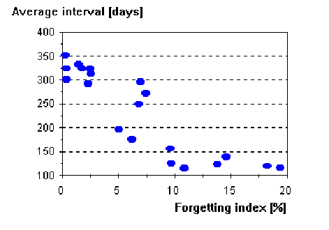
Figure 7 Scattergram illustrating the correlation between the forgetting index and the average interval
- average E-factor ranged from 2.464 to 2.706 (2.61±0.07), and was poorly correlated with examination results (correlation coefficient -0.11) [The concept of E-factor in Algorithm SM-6 corresponds roughly to A-factors in Algorithm SM-11]
- average number of repetitions ranged from 2.29 to 3.36 (3.0±0.27), and was poorly correlated with examination results (correlation coefficient -0.11).
- average number of memory lapses ranged from 0.01 to 0.65 (0.17±0.17). The positive correlation coefficient between examination results and the number of lapses was 0.34. Successful students would forget items more often (0.22 lapses per item on average) than unsuccessful students (0.09 lapses). For obvious reasons, lapses have been strongly correlated with the forgetting index (correlation coefficient 0.95), and with the average interval (correlation coefficient -0.78).
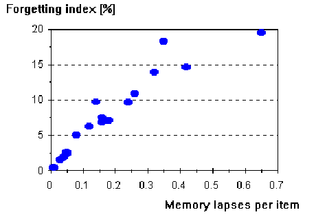
Figure 8 Scattergram illustrating the correlation between the average number of memory lapses per item and the forgetting index
- forgetting index ranged from 0.3% to 19.4%, its average value was 7.0%, and standard deviation 5.8%. Once again, successful students showed a greater degree of forgetting, with average forgetting index equal to 9% as opposed to 4% in the case of unsuccessful students (correlation coefficient equaled 0.42). As it was noted earlier, both response time and the forgetting index are slightly correlated with the examination result; hence the correlation coefficient of 0.39 between forgetting index and response time (see the figure). Again, these were students that gave their responses more consideration (more time) and judged themselves more critically (higher forgetting index) who were more successful in the examination.
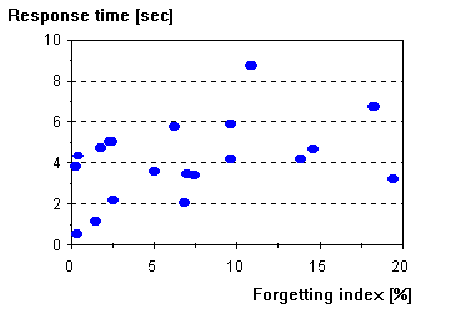
Figure 9 Scattergram illustrating the relationship between the forgetting index and the response time
- average grade ranged from 4.12 to 4.999 (4.8±0.2) and showed remarkably little correlation with the examination result (correlation coefficient -0.14)
- only six students had items with E-factors equal to 1.3. There was little correlation between the number of intractable items and the examination result
- the average difference between neighboring entries of the optimal factor matrix for the first repetition was 0.93 (ranging from 0.03 to 1.44). This difference was notably correlated with the examination result (correlation coefficient -0.5). The most likely interpretation of this fact is that bad students used to overestimate their grades. Consequently, little or no data was available to estimate optimal factors for low E-factors, while the optimal factor for the entry corresponding with E-factor equal to 2.5 was unnaturally high. A strong support for this interpretation comes from a very high correlation between the forgetting index and the average difference between optimal factor matrix entries in question (-0.9).
- as in the previous point, a very strong correlation has been found between the forgetting index and the O-factor value for E-factor equal to 2.5 and repetition number equal to one (correlation coefficient -0.89). Similar, though less pronounced correlation occurred for other entries of the matrix of optimal factors.
Because of my long-lasting interest in the approximation of forgetting curve and the nature of forgetting itself, I expected to collect valuable evidence for the exponential nature of forgetting by compiling a cumulative forgetting curve for E-factor equal to 2.5 and repetition number equal to one. Data from student file records have been superimposed to plot the average forgetting curve for items that enter the learning process. As it can be seen, the very high retention at repetitions rendered the collected evidence far from conclusive; despite a very large number of repetition cases gathered (over 51,000 repetitions in total).
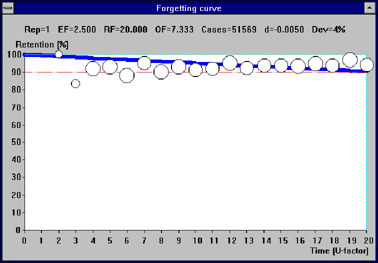
Figure 10 Cumulative forgetting curve for 20 students, E-factor 2.5, and repetition 1 (over 51 thousand repetitions collected)
In the presented figure, RF stands for R-factor, OF - O-factor, Cases - number of repetitions studied, d - forgetting decay constant from the equation retention=exp(-d*U-factor)), Dev - mean square deviation of experimental data from the retention curve approximated with the decay constant d.
A disappointing shortcoming of the assumed approach was a very high standard deviation of the detected forgetting index as reported earlier. As it is illustrated in the next figure, superposition of forgetting curves for different values of the forgetting index results in a U-shaped curve that shows little relevance with the true nature of forgetting (see Figure 11 Distorted forgetting curve resulting from differences in the forgetting index).

Figure 11 Distorted forgetting curve resulting from differences in the forgetting index
The U-shaped forgetting curve results from the fact that subjects with different values of the forgetting index, repeat items at different intervals, but the algorithm will always strive to make them forget no more and no less than the desired proportion specified by the forgetting index. This way, all students with intervals less than the maximum U-factor will tend to contribute to the forgetting curve around the point specified by the optimal interval, and their average retention, expressed in percent, will oscillate around 100 minus the forgetting index. Only the students whose intervals approach the maximum U-factor will show higher retention. Similarly, the highest retention will be registered for the shortest intervals; hence the U-shaped curve.
A 3-D representation of the cumulative matrix of retention factors is presented below (Figure 12 Cumulative matrix of retention factors). The matrix was obtained by superimposing forgetting curves corresponding with all R-factors taken from particular subjects.

Figure 12 Cumulative matrix of retention factors
In the figure presented above, the XYZ axes correspond respectively to the value of E-factor (from 1.3 to 3.2), repetition number (from 1 to 20), and to the value of R-factor expressed as percent of its maximum value. Note that for the sake of graph clarity, R-factors corresponding to repetition number greater than 2 were multiplied by 0.66 to expose the further located and more accurately estimated areas. The plain flat and plain down-sloping areas correspond to no repetition data available; hence they refer only to the model of average student (Wozniak et al. 1994). As opposed to the matrix of optimal factors, the figure illustrates a sharp contrast between the value of R-factors, and consequently the length of inter-repetition intervals across the range of E-factors. This contrast is marked, however, only for low repetition number. Because of the data collecting period limited to about 12 months, very few repetitions have been recorded in the area above the 3-rd repetition; hence much less visible differentiation of R-factors for different E-factor categories.
As the graphic presentation of the cross-section of retention factor matrices would require four dimensional figures, below I present such a cross-section flattened at the repetition number dimension. Thus, only the entries corresponding to the repetition number equal to one are presented.
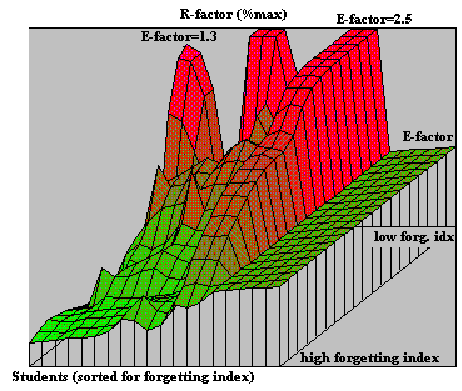
In the figure presented above, the XYZ axes correspond respectively to the value of E-factor (from 1.3 to 3.2), subject number (subjects were sorted for forgetting index; lower values placed distally), and to the value of R-factor expressed as percent of its maximum value, which is 20 in the case of first repetition. The plain flat area corresponds to no repetition data available.
The down-sloping ridge corresponding with E-factor equal to 2.5 illustrates the influence of the forgetting index detected during repetition on the value of R-factors. The two peaks located at E-factor=1.3 and E-factor=1.8 illustrate the saltatorial flow of items down the E-factor axis in result of forgetting. The peaks result from high retention detected at repetitions of the forgotten items. The valleys placed in-between, do not indicate the inherently irregular nature of the matrix of R-factors, but show only the areas, where low number of repetition cases prevented establishing the accurate value of the matrix entries. The three-peak nature of the first row of the matrix of retention factors corresponding with repetition number equal to one disappears with the progression of the forgetting index toward higher values. Though the above observation might suggest adopting a sparser matrix of R-factors with fewer E-factor columns, the situation presented in the figure is not necessarily typical. The location of peaks, or even their appearance will greatly depend on the student’s grading habits, which influence the rate of change of E-factor values.
As in the case of cross-section of retention factor matrices, a cross-section of optimal factor matrices flattened at the repetition number dimension is presented below (Figure 14 Comparison of O-factors for repetition number equal to one). Only the entries corresponding to the repetition number equal to one are presented.
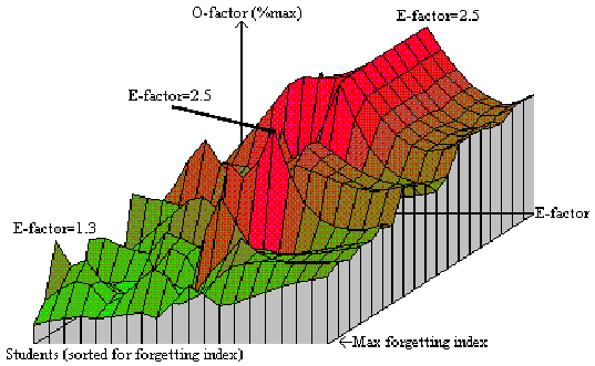
Figure 14 Comparison of O-factors for repetition number equal to one
In the figure presented above, the XYZ axes correspond respectively to the value of E-factor (from 1.3 to 3.2), subject number (subjects were sorted for forgetting index; lower values placed distally), and to the value of O-factor expressed as percent of its maximum value, which is 20 in the case of first repetition.
As the matrix of optimal factors is derived directly from the matrix of retention factors, a natural correspondence can be seen between the shape of the cross-analysis graph for O-factors and repetition number equal to one and the same graph for R-factors (cf. Figure 13 Cross-comparison of R-factors for the first repetition and varying E-factor among the subjects sorted for the forgetting index). The steady decrease of O-factors between the ridge at E-factor=2.5 and higher E-factor areas, in marked contrast to the same region in the corresponding R-factors graph, results from the application of on-line smoothing of the matrix of optimal factors in the process of learning. Analogously, the two peaks discussed in the case of R-factors comparison blended with the surrounding area providing for more regular spacing of repetitions across the E-factor matrix.
Yet more conclusive is the same graph plotted upon weighted Gaussian smoothing of the 3-dimensional matrix of optimal factors, i.e. the matrix built from optimal factor matrices extended by the student dimension. The weight used in Gaussian smoothing was the number of repetition cases recorded.

Figure 15 First layer of the 3-D matrix of optimal factors upon weighted Gaussian smoothing based on the number of repetition cases
In the graph presented above, which is a smoothed equivalent of the one presented earlier (see Figure 14 Comparison of O-factors for repetition number equal to one), it can be more clearly seen that three elements determine the value of the matrix of optimal factors for repetition number equal to one:
- students with high forgetting index show lower and less differentiated range of values in the first row of the matrix of optimal factors
- optimal factors are correlated with the value of E-factor, and increase faster for lower values of the forgetting index (except E-factors greater than 2.5)
- because of a very low number of repetition cases for E-factors greater than 2.5, the first row of optimal factor matrix beyond E-factor equal to 2.5 is determined almost exclusively by on-line smoothing that makes part of the Algorithm SM-6
For low forgetting index, a particularly large difference between O-factors for E-factors equal to 2.5 and E-factors less than two, results not only from an inherently longer inter-repetition intervals for easier items, but also from the slower convergence of O-factors to their optimal value at low E-factor areas due to reduced number of repetition cases which drive the optimization.
Comparison of the distribution of intervals in particular subject file records shows that, for natural reasons, students with low forgetting index show less differentiation among item intervals, and that the average interval is greater. For example, the least successful students, with the lowest value of the detected forgetting index showed the greatest number of items in the 256-512 days slot. On the other end of the spectrum, the mode of distribution for the highest forgetting index coincided with the 64-128 days interval range (see Figure 16 Comparison of inter-repetition interval distribution among students sorted for forgetting index).
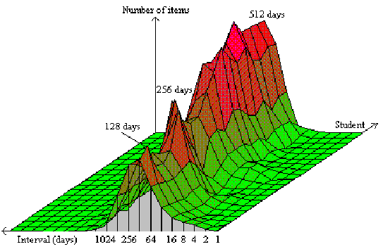
In the above graph, the XYZ axes correspond respectively to the interval category (note, that for the sake of graph clarity, the polarity of the axis was reversed), subject number (subjects were sorted for forgetting index; lower values placed distally), and to the number of items falling into the particular interval category (the Z line has not been calibrated because of its dependence on the size of the question-answer list).
As in the case of interval distribution, students with high forgetting index showed an increased differentiation of E-factors, though the mode of the distribution did not indicate greater difficulty of items among the students with higher forgetting rates. [The concept of E-factor in Algorithm SM-6 corresponds roughly to A-factors in Algorithm SM-11]
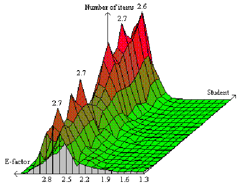
Figure 17 Cumulative distribution of E-factors among students sorted for forgetting index
In the presented graph, the XYZ axes correspond respectively to the E-factor category (note again, that for the sake of graph clarity, the polarity of the axis was reversed), subject number (subjects were sorted for the forgetting index; lower values placed distally), and to the number of items falling into the particular interval category (the Z line has not been calibrated because of its dependence on the size of considered databases).
The most striking observation coming from the comparison of E-factor distributions is that the tested list of questions and answers appeared to be surprisingly easy for all subjects. As a consequence, the graph shows a uniform ridge along the E-factor category of 2.6-2.7, and there is no perceptible bulging around the 1.3 category, which in most cases acts like a scavenger of bad items, and can be used in implementing programmatic filters that make it possible to eliminate ill-structured items from lists of questions and answers.